How isochrones work: From shortest paths to polygons

In this post, I'll walk you through the mathematics behind isochrones. We'll start with how a road network is modeled as a weighted, directed graph. Then we'll run Dijkstra's shortest path algorithm to compute the travel time from a source node to every other node in the network. Applying a cutoff (the isochrone's time limit) leaves us with the set of reachable nodes and their distances. Since those distances live on the graph rather than in the plane, we resample them onto a grid to build a cost surface, then run marching squares over it to cleanly trace the isoline: the boundary of the isochrone polygon.

Part 1: Mapping travel time with the Google Maps Isochrones API
Part 2: How isochrones work: From shortest paths to polygons (this article)
Part 3: Build a travel time map using the Google Isochrone API

What is an isochrone?

An isochrone is a line, or the area it encloses, connecting all the points you can reach from a starting location within a fixed amount of time. It's used widely in commercial site selection (deciding where to open a new store), real estate and urban planning (making sure that new building or neighborhood is accessible to grocery stores and other amenities) and logistics (determining whether an address falls within a service area).

Why use isochrones?

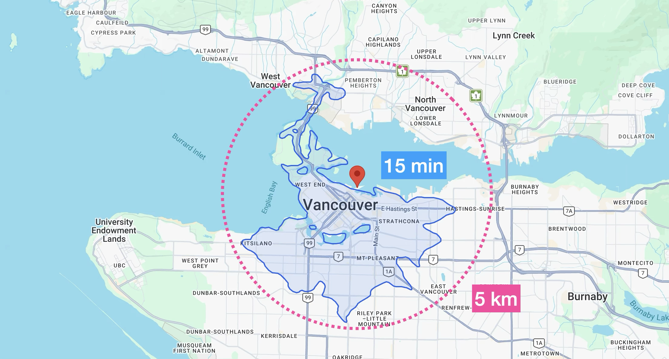
An isochrone gives you a far better picture of what's actually reachable than a simple x kilometer radius. A radius just draws a circle as the crow flies; an isochrone follows the road network and accounts for how people really travel by car, on foot, or by bike, each at its own speed. The map above makes the gap obvious: much of the area inside a five kilometer radius can't be reached within 15 minutes of driving.

More formally, an isochrone is the boundary of everywhere you can reach from a starting point s within a set time T, measured along real roads rather than using straight line distance.

How do you build an isochrone?

In general, there are five main steps to building an isochrone:

1. Model your road network as a weighted, directed graph where nodes are intersections, edges are road segments and edge weights are travel times.
2. Run Djikstra's to compute travel times from s (source node) to every other node in the graph.
3. Terminate the search once the total travel time to a node exceeds T.
4. Resample the graph onto a raster grid and use marching squares to cleanly trace the travel time boundary (the isoline).
5. Fit a smooth curve through the isoline using a spline smoothing algorithm such as Chaikin's algorithm.

I'll walk through each of these steps in detail, then close with a look at what makes each one hard in practice, and how those challenges shape which isochrone API is right for you.

Model a road network as a weighted directed graph

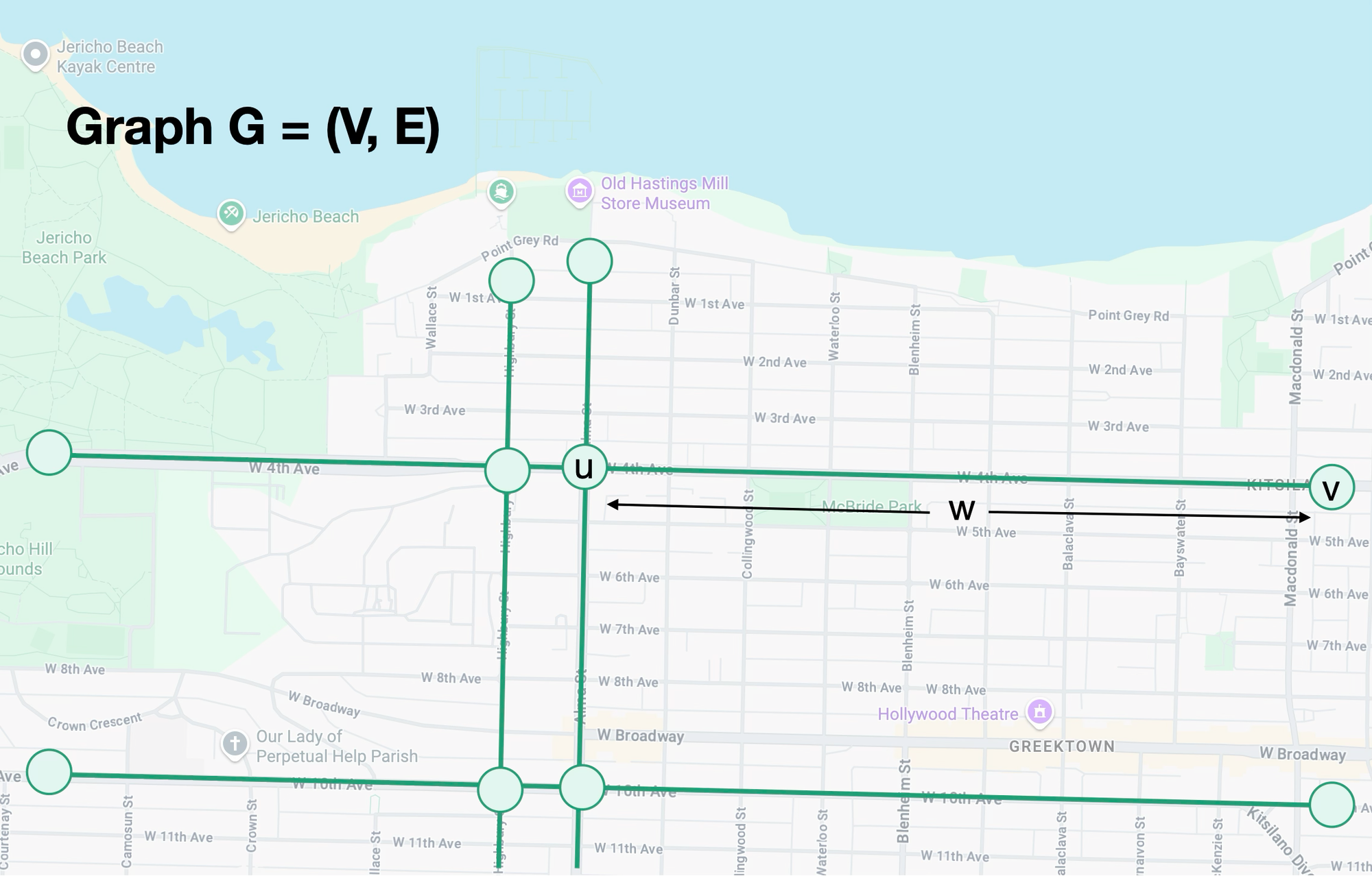
In mathematics, a graph G = (V,E) is a structure containing V, a set of vertices (also called nodes) and E is a set of edges, each edge joining a pair of vertices. In a directed graph, an edge is written as a pair of vertices, e = (u, v), and the two vertices it joins are called adjacent. They're neighbors, directly connected by that edge. In a weighted graph, each edge also carries a weight, written w(u,v): a number giving the cost of that connection. This could be the distance, travel time, or anything really, so that w(u,v) is the "length" of the link between adjacent nodes u and v. For isochrones and routing, that weight is travel time (the segment's length divided by its speed) which shifts with the time of day (traffic) and the travel mode (walking, cycling, or driving).

A road network maps to a graph almost one to one, which is what makes graph algorithms the natural tool for routing and isochrones.

Compute travel times using a shortest path algorithm

With the graph in place, the next step is to compute the shortest travel time from our starting location (the source node s), to every other node in the network, stopping as soon as those times exceed the travel time budget T.

To get there, I'll walk you through Dijkstra's shortest path algorithm. It's one of the most famous algorithms in computer science (and surprisingly easy to understand). Yet it's the workhorse behind the routing engines used by Google Maps and other mapping providers. Here's how it works.

Initialize a distance value for every node, setting the source (node 1) to 0 and all others to infinity, and mark every node as unsettled. Then, while any unsettled node has a finite distance, select the unsettled node with the smallest current distance and call it the current node. Settle it. Its distance is now final and will never change. For each edge leaving the current node to an unsettled neighbor, compute a candidate distance as the current node's distance plus that edge's weight; if the candidate is smaller than the neighbor's stored distance, overwrite the neighbor's distance with the candidate. Repeat until no unsettled node remains reachable.

Because edge weights are non-negative, the moment Dijkstra finalizes a node it has already found that node's shortest distance. No later path can beat it, which is why it's provably correct.

Halt once the nearest unsettled node exceeds the travel time budget T

Recall that an isochrone is the area containing every point reachable from a starting location within a fixed amount of time. To turn Dijkstra's search into an isochrone, we stop as soon as the nearest unsettled node exceeds the travel time budget. Because Dijkstra settles nodes in nondecreasing order of travel time, once that nearest unsettled node is over budget, every remaining unsettled node must be too, so there's nothing left worth searching.

But in practice, the travel time budget almost never runs out exactly at a node. Say a node sits at 12 minutes under a 15-minute budget. You can still travel three more minutes down each road leaving it before the budget expires. So the true boundary of the isochrone lives mid-edge, not at the intersections.

To find it, take each edge that leaves a within-budget node and would overshoot the limit, and figure out how far along it you get before the time runs out. With the remaining budget (3 minutes) and the edge's cost, you compute the fraction of the edge you can cover and linearly interpolate a point at that spot along the edge's geometry. Those interpolated points are the real frontier, which is what is shown in the interactive visualization above.

Note: Since an edge can be partly reachable from either end, you need to interpolate each edge from both of its in-budget vertices, not just the one you happened to settle first.

Resample the graph onto a raster grid and run marching squares to trace the travel time boundary

To turn the travel time graph into an isochrone, we need to first convert the graph into an area by rasterizing it i.e. overlaying a grid over the map and give each cell a travel time value interpolated from the nearby nodes and edges. That turns the sparse graph into a continuous cost surface which is exactly what marching squares (a well known contouring algorithm, more on this later) needs to trace a boundary.

With the grid overlaid, we give every grid point (the cell corners) a number: an estimate of the travel time from the source to that point. We derive that from the network distances Dijkstra already gave us, plus a penalty for however far off-road you'd have to go to reach that point. Now marching squares can run: it compares each cell's corner values against the budget T and traces the boundary line wherever a cell has some corners inside the budget and some outside. That traced line is the isochrone. In the visualization above you can adjust the travel time budget to see how that affects the isoline.

Fit a smooth curve through the isoline

The raw isoline that marching squares hands back is jagged, with a visible corner at every grid boundary. That's geometrically faithful but it doesn't look like the clean shape people expect on a map, so the final step is to smooth it.

Rather than pass a curve through hundreds of vertices, we round the corners with a spline smoothing algorithm such as Chaikin's algorithm, which repeatedly cuts each corner in two and replaces every sharp vertex with a pair of points slightly along its edges, so that after a couple of passes the staircase relaxes into a smooth, natural looking boundary. The result is the polished isochrone we're all familiar with.

The visualization above should give you some idea of how this works. The teal boundary is what Chaikin gives you at the current iteration count, and each pass roughly doubles the vertex count because corner cutting replaces every point with two new ones slightly along its edges. Diminishing returns kick in fast. Between 0 and 2 iterations the change is dramatic; past 3 or 4 it's barely perceptible but the vertex count keeps exploding. For a real renderer you'd stop at 2 - 3.

So should you write your own isochrone map generator?

Yes and no. I've shown you the fundamentals of how isochrones are built, but running and maintaining your own isochrone generator is a serious undertaking. You'd need a server with enough memory to hold the entire road network graph, and enough compute to run Dijkstra's and return a smoothed isochrone in a few hundred milliseconds or less - fast enough to feel instant.

That said, if you're working with your own small, custom network, one whose vertices and edges aren't well captured by the general road network, building your own isochrone generator could be a genuinely useful and fun project.

That said, if you're working with your own small, custom network, one whose vertices and edges aren't well captured by the general road network, building your own isochrone generator could be a genuinely useful and fun project.

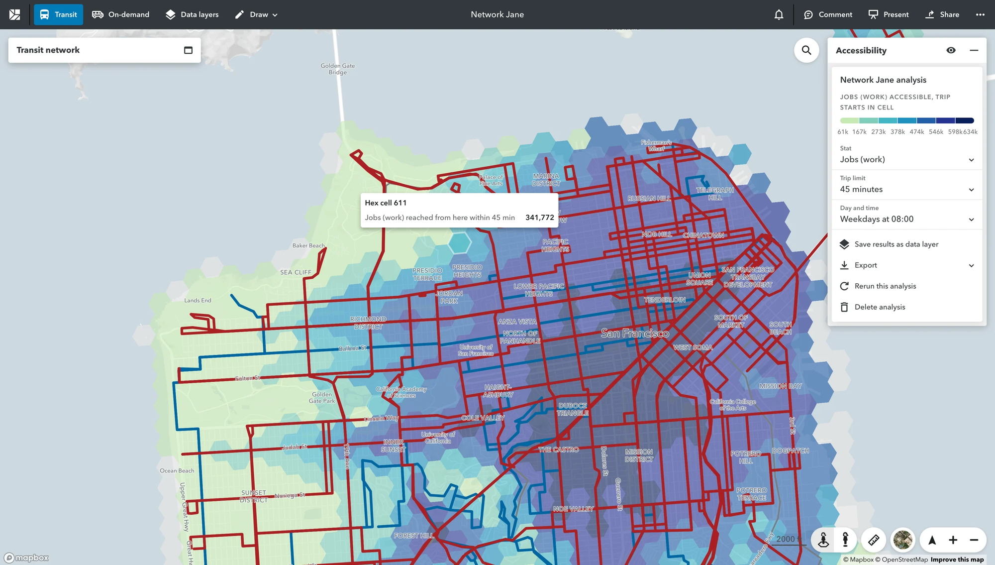
A good example is Remix's Jane, a travel time isochrone that shows how far a person can get from a chosen point within a set time. Remix, a collaborative mapping and planning platform now part of transit provider Via, is used by transit agencies across the US to build transit networks and schedules from scratch. Because that network data is theirs alone, it won't exist on Google or OpenStreetMap, so it makes sense for them to build their isochrone generator in-house rather than depend on a third party API.

What should you look for in an isochrone provider?

Now that you have a better understanding of how isochrones are made, let's review what makes a good isochrone API.

Since every isochrone starts from a graph of the road network, choose a provider whose map is a detailed, up to date representation of the world and whose traffic model reflects how people actually drive. The Google Maps Isochrones API is a clear winner here, but other providers such as HERE Maps have excellent road network coverage as well.

As we've seen, the workhorse behind any isochrone is Dijkstra's shortest path algorithm. In practice, though, running a full Dijkstra search over a city scale road network for every request is too slow at volume. So production routing engines precompute much of the work ahead of time, using techniques like contraction hierarchies to collapse the search space dramatically. Regardless of what method is used, you should choose an isochrone provider that returns good looking isochrones as fast as possible. The TravelTime Isochrone API is currently the fastest based on publicly available benchmarks. Keep in mind, though, that "fast" is relative. If isochrones are one step inside a route optimization loop, they need to be very fast. Other calculations are waiting on the result. But if you're just showing the walkable area around a property, speed barely matters. The page can load the isochrone asynchronously, after the main content is already on screen.

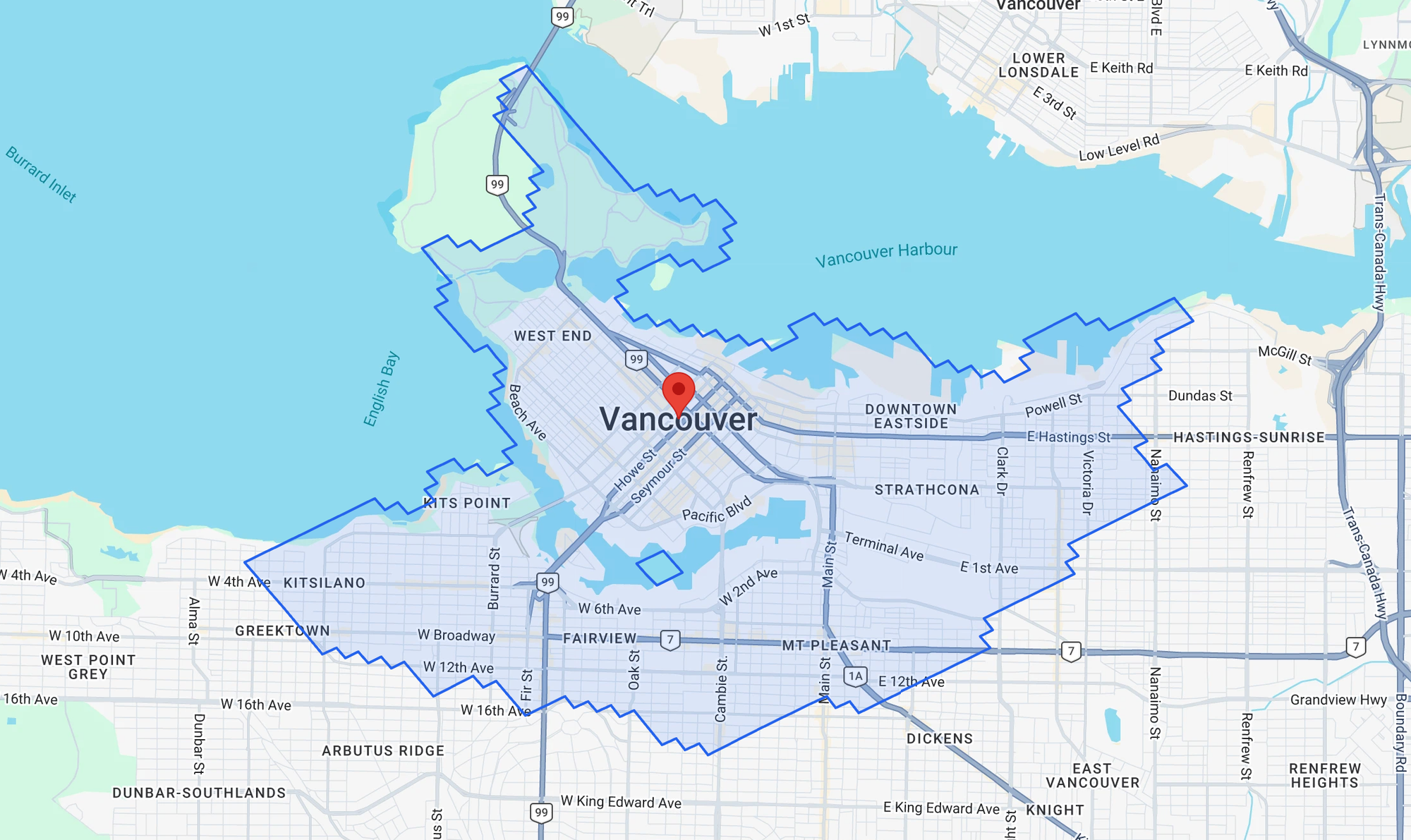
Lastly, you might want to choose a provider that lets you trade run time against isochrone quality. Just as we saw how marching squares produces jagged isochrone boundaries, you may sometimes want a provider like Google that lets you skip the boundary smoothing step when speed matters more than a polished shape.

This article was written by Afi Labs, a Google Maps Premier Partner and reseller. We build route optimization, navigation, and fleet tracking software on Google Maps, and offer volume pricing on GMP licensing. Talk to an engineer or follow Afian on LinkedIn.

Next: Part 3: Build a travel time map using the Google Isochrone API